Saturday, August 31, 2013
Friday, August 30, 2013
How to use Slicer for effective filtering of Pivot Data in MS Excel?
About Slicers in MS Excel
Slicers provide buttons that you can click to filter PivotTable data. In addition to quick filtering, slicers also indicate the current filtering state, which makes it easy to understand what exactly is shown in a filtered PivotTable report.Step 1: To get the Slicer option you have to go the "Insert" Ribbon's "Filter" tool. There you will have two options 1) Slicer and 2) Timelines.

Step 2: Create you pivot table and then click Slicer. You will get the Slicer selection list.
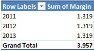
Step 3: Select the Year and Margin or all three. You will get the slicer of your pivot table.


Subscribe to:
Comments (Atom)
-
 The Ribbon is designed to help you quickly find the commands that you need to complete a task. Commands are organized in logical groups, whi...
 -
 Contextual tabs gets activated when you create SmartArt, chart, drawings, picture, header and footer, Ink, Sparkline's, timeline, slicer...
 -
 Many a times you do some calculations in a spreadsheet or prepare a small report for some use. After creating that, either you realize that ...